Dataviz Challenge #3: The Side by Side Bar Chart

1 Reply

Thanks to everyone who participated in the first and second dataviz challenges! I hope these challenges give you a chance to practice and build upon your Excel and visualization skills.

Last time, we made a streamlined version of the basic bar chart by adjusting Excel’s default settings. Basic bar charts are great when you’re just looking at simple patterns, like one series of data at a time.

However, sometimes we need compare several series of data at one time. For example, the Innovation Network team and I recently compared the capacity of 12 different coalitions using our coalition assessment tool. We calculated coalition capacity in 7 different areas, such as Basic Functioning and Structure and the Ability to Cultivate and Develop Champions. To learn more about the tool, check out some materials from a recent presentation here.

The “before” chart: Here’s a clustered (aka cluttered) bar chart based on fictional data from the coalition assessment tool. The default Excel chart to compare Coalition A and Coalition B might look something like this:

A default clustered bar chart in Excel. Bleh.

Or, you could use the switch row/column feature to make a default chart like this:

Another default clustered bar chart in Excel.

These default clustered bar charts work… kind of. Well… not really. Actually, no, they really don’t work at all! My brain needs a couple minutes to read the default charts and really think about comparisons.

The “after” chart: Luckily, with a little Excel elbow grease, we can make the patterns pop out even faster. Here’s a side by side bar chart:

Now, my brain can see the patterns almost immediately: Both coalitions scored highest on Basic Functioning and Structure. Both coalitions scored lowest on Sustainability, with Reputation and Visibility scoring pretty low as well. Coalition A scored higher than Coalition B on every section of the assessment. The overall scores were 80% for Coalition A and 50% for Coalition B. Phew! This is much easier for my brain.

The dataviz challenge: Re-create the “after” version of the side by side bar chart in Excel, R, or some other free software program. When you’re finished, email me or tweet a screenshot to @annkemery.

Tips for beginner Excel users: First, learn how to make a basic bar chart. Then, check out this powerpoint for tips on making a side by side bar chart.

Bonus for advanced Excel users: Instead of copying this dataset exactly, think about how you might use a side by side bar chart in your own work. Can you re-create this chart using your own data or your own color scheme?

The prize for playing: Beer or coffee, my treat, the next time you’re in DC; a professional development opportunity; and bragging rights.

I’ll post the how-to guide in two weeks, on June 7, 2013. Happy charting!

Dataviz Challenge #2: The Answers!

8 Replies

Two weeks ago, I challenged readers to re-create the “after” version of a basic bar chart. You can read the full post here.

Congratulations to the 9 winners: Molly Hamm, David Napoli, Susan Kistler, Jon Schwabish, Ethan, Mike, Sara Vaca, Samantha Grant, and Kevin Gilds! You’ve officially won bragging rights and a beverage of your choice, my treat, the next time you’re in DC.

Now it’s time to post the how-to guide!

Step 1: Study the chart that you’re trying to reproduce in Excel.

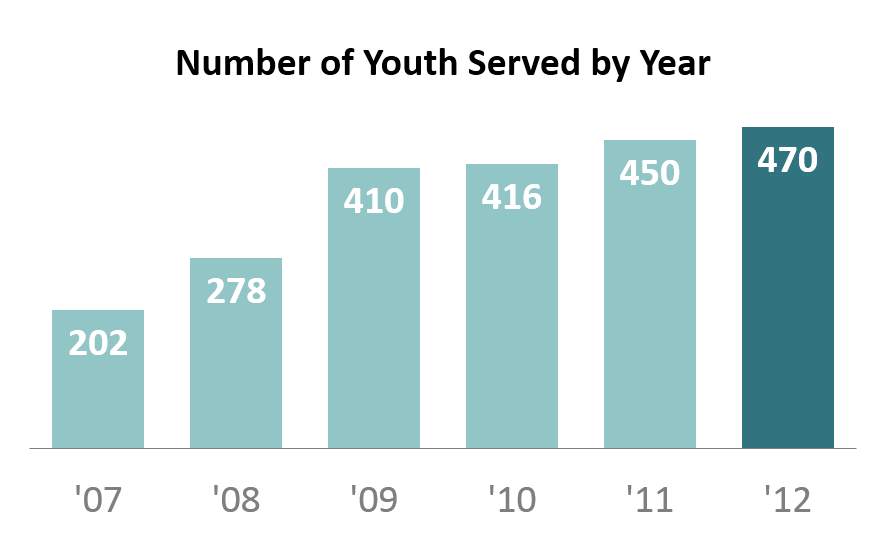
We’re trying to re-create a basic bar chart like the one shown below. We’re examining how a nonprofit has grown over the past six years. This is a simple metric so we don’t need anything more complicated than a basic bar chart.

Step 2: Type your data into Excel.

Here’s how I typed my data into the spreadsheet.

Hot tip for advanced users: I wanted to abbreviate the years (i.e., ’07 instead of 2007). If you type 07, it will turn into 7, because Excel automatically removes zeros at the beginning of numbers. To fool Excel into keeping the zero, you must add an apostrophe; typing ’07 will turn into 07. So, if you want to get ’07 as your final result, you must add two apostrophes; typing ”07 will turn into ’07.

Step 3: Insert a bar chart.

Highlight or select the data table. Go to the Insert tab. Click on the Column icon. Select a 2-D Clustered Column Chart. For additional help with inserting charts, check out this tutorial.

Now we’ve got our default bar chart (shown below). There’s nothing technically wrong with this bar chart. However, with a few small tweaks, we can really improve the formatting.

We’re going to manually adjust 9 settings in Excel: the axis labels, the data labels, the border, the bar color, the font size and color, the gap width, tick marks, the legend, and the grid lines. We’ll go through each of these steps, starting with the axis labels and working around counter-clockwise. These tweaks just take a few seconds each to make. When added together, they can make a big difference.

Step 4: Delete the axis labels.

Click on the axis labels themselves. Then press delete on your keyboard. I do not advocate for removing the axis labels on every chart. This is a matter of personal preference. In this example, the data are so ridiculously straightforward that we really don’t need the axis labels.

Step 5: Add data labels.

Data labels are the numbers inside the bars that show how many participants were served each year. To position the data labels inside the bars themselves, we need to use a 2-step process. First, right-click on one of the blue bars and select “Add Data Labels.” Second, right-click on one of the labels and select “Format Data Labels.” You’ll get a pop-up screen like the one shown below. You can tweak the label position. In this example, I selected “Inside End.” Then, you can simply click on one of the data labels and change the text color to white. For more help with data labels, watch this tutorial.

Step 6: Remove the border.

Right-click on the border and select “Format Chart Area.” Click on “Border Color” and select “No Line.”

Removing the border is also a personal preference. I started deleting my borders after reading one of Edward Tufte’s books in which he advocates for charts being situated inside and alongside the narrative – rather than sticking charts in the appendix or adding awkward “Figure 1.4″ labels. Border-less charts tend to help the reader’s eyes glide down the pages of your report a little more seamlessly.

Step 7: Adjust the bar color.

This chart was originally designed for an Ignite session. You can view the slides here.

After giving the presentation, there were a few audience questions. One man, with his (first? second? third?) glass of wine in his hand, asked how I selected the turquoise color scheme. He was laughing (with me? at me?) because I was wearing a dark turquoise shirt, a light turquoise blazer, a turquoise necklace, a turquoise bracelet, and turquoise earrings. Yes, even my toenails were painted turquoise. I mumbled something like, “I guess I just really like turquoise!” and promptly ran off the stage. #npfail

The correct answer would’ve been that colors should be used strategically so that the reader’s eyes are naturally drawn to certain patterns in the data. For example, I purposefully drew the reader’s attention to the 2012 bar. The key is to select a plain color (e.g., gray, or light turquoise in this example) and what Stephanie Evergreen calls an action color (e.g., dark turquoise). For examples of plain colors and action colors, check out Stephanie Evergreen’s post on assigning a color system for graphs.

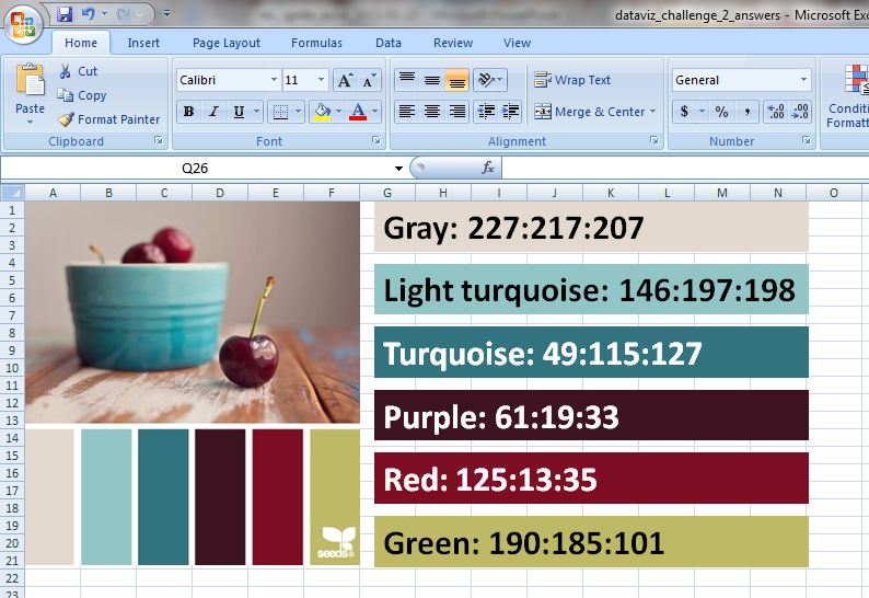
I like to professionalize my charts by tweaking Excel’s default color scheme. During fun projects like this, I select color schemes from Design-Seeds and use the Instant Eyedropper to determine each color’s RGB code. I selected the Cherry Palette for this Ignite presentation (shown below). During real projects, I match colors to the client’s logo.

Sometimes I save my color palette and RGB codes within the Excel workbook itself for safekeeping and easy reference.

So how do you adjust the bar color? Click on one of the bars. Click on the paint can icon. Select “More Colors.” In the pop-up window, select the “Custom” tab. Type in the RGB codes for your plain color and the action color.

Step 8: Adjust the font size and colors.

Here’s another spot where personal preferences come into play. When I’m going to be pasting my chart into a report, I often match my chart’s font to the report (e.g., Calibri size 11, which we typically use for the body text). When I’m going to be pasting my chart into a single, standalone handout, or into a powerpoint slide, I use much larger font sizes (e.g., 14, 16, or 18 point font). When I’m using data labels within the bars (see Step 5), I often use bold font to make the text pop.

Gray can be used strategically to dull-down the least important features of the chart – like the horizontal axis labels (’07, ’08, ’09, ’10, ’11, and ’12).

We’re getting closer! Not there yet…

Step 9: Adjust the gap width.

Gap width is a lesser-known, but very cool, feature of Excel. The gap width is the amount of space between the bars. The default setting on most computers is 150%, which means the distance between the bars is 1.5 times wider than the bar itself.

To adjust gap width, right-click on one of the bars and select “Format Data Series.” In the pop-up window, you can increase or decrease the gap width, as shown below. I often use 50-75% rather than the default 150%.

Hot tip for advanced users: The gap width feature is also very useful for histograms. You can decrease the gap width to 5% so that only a sliver of space remains between the bars.

Step 10: Remove tick marks.

For help with tick marks, watch this tutorial.

Step 11: Remove the legend.

In this simple chart, the legend doesn’t serve any purpose. To remove the legend, simply click on the legend and press the Delete key on your keyboard.

Step 12: Remove the grid lines.

Again, because this chart is so simple, we don’t need the grid lines. For help removing the grid lines, watch this tutorial.

We’re all done! Here’s the finished product.

Step 13: Add a caption (optional).

Charts are inserted into a variety of communications modes: within the body of a report, as a standalone chart that’s printed out and hung on a bulletin board, as a standalone chart that’s printed and used as the handout at a meeting, on a powerpoint slide…

This particular chart was flashed on the screen for 15 seconds during my Ignite session, so there was no need to add a caption. My voice served as the caption.

However, when creating standalone charts, you’ll want to add contextual details so that the reader who passes by your chart on your organization’s bulletin board can quickly grasp the chart’s key takeaway message. One of the best ways of adding contextual details is to add a caption within the Prime Real Estate at the top of the chart. For an example, check out this post by Cole Nussbaumer.

Bonus

I hope this was helpful! Click here to download my Excel file. Thanks again to the dataviz challenge winners, Molly Hamm, David Napoli, Susan Kistler, Jon Schwabish, Ethan, Mike, Sara Vaca, Samantha Grant, and Kevin Gilds!

Discussion Questions

What are your favorite tools for selecting color palettes and determining RGB codes? When do you add captions to your charts, and what are your strategies for selecting the most important findings to emphasize in that caption? Have you adjusted the gap width for any of your charts, and if so, in what situations?

Dataviz Challenge #2: The Basic Bar Chart

18 Replies

The first dataviz challenge was a hit! A few of you wanted to participate but weren’t ready to jump into a challenge that required so much Excel elbow grease. So, this second challenge is geared towards beginners like you. Once I build your foundational skills, we’ll move on to advanced charts.

I’m giving an Ignite presentation tomorrow at the Nonprofit Technology Conference (#13NTC). I’m going to show nonprofit leaders how to make four easy-to-read bar charts by simply using a little #ExcelElbowGrease:

First, let’s take a closer look at default Excel bar charts. The “before” bar chart is shown below. In my example, we’re examining how a nonprofit has grown over the past six years. This is a simple metric so we don’t need anything more complicated than a basic bar chart.

You’ve probably seen these exact charts before. There’s nothing technically wrong with this default bar chart. It doesn’t distort the data. It doesn’t mislead the readers. Default charts are fine for internal use like informal staff meetings. However, a few tweaks can really improve the formatting.

The “after” chart is shown below. Now, my brain sees the pattern immediately. There are fewer distractions — no border, no tick marks, no grid lines. In other words, this bar chart passes the Squint Test — when you squint your eyes, and everything gets a little blurry, you should still be able to detect the overall shape of the data. There shouldn’t be extra ink like borders, tick marks, or grid lines getting in the way.

I also infused a few of my personal preferences into the chart’s formatting. My eyes do better with the larger font. Being a data nerd, I prefer having data labels on my bars so I can read the exact values (rather than having to estimate values in the default chart). The white space and custom color palette make the chart look like something a graphic designer might create. I purposefully focused attention on the 2012 bar by using a darker color. Like I mentioned, these last few adjustments aren’t required. Passing the Squint Test is more important than satisfying everyone’s personal preferences. There are multiple correct ways to improve chart formatting.

The dataviz challenge: Re-create the “after” version of the basic bar chart in Excel or R. No expensive software allowed. You can re-create this exact bar chart, or you can tweak the color scheme and numbers to fit an example from your own work. The goal is to practice manipulating the settings in Excel and to create a basic bar chart that’s easy to read and understand. When you’re finished, email me or tweet a screenshot to @annkemery.

Bonus: Beginners can probably make this bar chart in 30 minutes or less (for example, during your lunch break). You’ll get faster with practice. I bet that advanced Excel users can enter the data, insert the chart, and adjust the chart in 3 minutes or less. Time yourself. Advanced users, how fast are you?

The prize for playing: Beer or coffee, my treat, the next time you’re in DC; a professional development opportunity; and bragging rights.

I’ll post the how-to guide in two weeks, on April 24, 2013. Happy charting!

The best Ignite presentations are when the presenter stumbles over words [Guest post by Kevin Flora]

4 Replies

Kevin Flora is an evaluator and blogger at edmatics.org who watched, recorded, edited, and uploaded all 56 Ignite sessions from the 2012 AEA conference.

Ignite sessions… a presentation format started by O’Reilly that I thought would never stick around. The more I conduct my own presentations, I feel as though the audience engagement and personal enthusiasm is a direct reflection of my content. If this theory holds true, then the Ignite format should be more prevalent due to its ease of producing laughs and forcing the presenter to stay on top of their information. Essentially, there are 20 slides. Each slide advances automatically every 15 seconds whether the presenter is ready or not. Are you doing the math? Yes, it’s a 5-minute presentation.

The one thing I love about this format is the first-time presenter! When initially signing up, the thought is, “How hard could this be? Five minutes? That’s easy enough.” Well… I have found that it takes just as long to prepare for these 5 minutes as it does a 45-minute presentation, if not longer. Everyone wants to look at notes or the presenter view on the PowerPoint screen, but the best presentations are when the presenter stumbles over words, gets behind (or ahead) on their timing, and forgets why he/she used a particular image in their slide deck. I have heard that the more Ignite presentations an individual does, the less interesting they are to the audience because of the ability to almost perfect the structure. These are meant to be fun, with pictures, stories, and yes… screw-ups once and awhile.

Ignite presentations can be used for multiple purposes. My favorite Ignite session was that of Michael Szanyi at the 2012 American Evaluation Association (AEA) conference. His use of interpretive dance brought the data visualization and reporting topical interest group (DVR TIG) to their feet and moved some to tears. Szanyi produced an unrivaled passion for how his form of art and expression should be used in visualizing data. Szanyi not only memorized his slides, but the timing, movement, and slide descriptions. After seeing his 5-minute production, I saw where the future of Ignite presentations and evaluation was headed. This glimpse of our future was a sight to see. Here is Szanyi’s presentation:

After watching 56 presentations, it is difficult to find a comparison to Szanyi’s performance, so I will mention a couple of other neat ideas. The DVR TIG conducted their entire business meeting with the 5-minute presentation format (watch them all here), milking cows was related to strategic learning (here), and an improv Ignite was attempted (which made for a hilarious 5 minutes. Thank you Chris Lysy). Check out Chris Lysy’s improv Ignite here:

The Ignite format is both interesting and fun… informative, but short… and effectively cultivates an atmosphere conducive to questions, collaboration, and further discussion on certain topics. All 2012 AEA Conference Ignite videos can be found on the AEA YouTube channel.

Connect with Kevin Flora through his blog at www.edmatics.org or @edmatics on Twitter!

Blog-o-versary!

7 Replies

Celebrating… my first blog-o-versary!

My first post was on March 23, 2012. A year ago, I was concerned that I wouldn’t have anything to blog about. Surprisingly, my biggest challenge has been trying to blog less frequently!

Looking Backwards

What’s worth celebrating? Here are a few milestones from the past year.

1 new job at Innovation Network (hence a blog name change)
2 podcasts
3-hour eStudy about dashboard automation
4 conference presentations at EERS and AEA
45 Excel tutorials
99 blog posts (67 from me on this blog; 8 on other blogs; plus 24 guest posts from 14 different colleagues)
1,000+ tweets at @annkemery
21,000+ blog views
1,000,000+ numbers crunched
Infinite connections with colleagues in the evaluation blogosphere

Looking Forwards

What’s to come in the next year?

More data visualization challenges. The first challenge was overwhelmingly popular. I’ll start with beginner-level challenges and work up to harder ones.
More Excel tutorials. I may add R tutorials later in the year.
More hands-on tips about surveys, dashboards, interviews, and focus groups. This bank of focus group questions, these ideas for interactive focus groups, and this comparison between focus group and meeting facilitation are some of the most popular posts. Stay tuned for more like these!
More posts about potent presentations
More guest posts

Thanks for reading! I’m glad I started blogging, and my only regret is that I didn’t start sooner. I hope to see many more evaluation blogs emerge over the next year.

Pivot Tables: Your Tool for Exposing Miscreant Data

9 Replies

Thank you, Ann Emery and thanks especially to the visitors of EmeryEvaluation.com. It meant a lot to be asked to do a guest blogpost because Ann’s approach is practical, focused on real-world experience, and her dedication to empowerment of others is a key theme at my own site, DataScopic.net.

I’ve been working with Excel and data for 15 years and developed a skill for scrubbing data. So, data quality is always on my mind. This year, I’m teaching more workshops so that others are empowered to manage their own data quality and develop sound spreadsheets.

Hopefully, you’ll find this blogpost useful. Please comment, ask questions and be in touch.

- Oz du Soleil

Today, we’re going to discuss data quality, messy data, or, as I’ve described in several blogposts, crap data. As a complement to this post, there is a dataset of 455 rows for us to work. Click here to download the sample dataset.

WE HAVE OUR DATA: What Do We Want To Know?

We want to dig in and find out things like:

Of the members we had in 2009, how many are still active members?
What were the 2010 donation amounts of the currently active vs. inactive members?
What were the 2008-2010 donations for the states where we plan to close offices: IN, MA and SC?
What were the 2008 donation totals of the Gold, Platinum and Lifetime members?
Are our Lifetime members clustered in a region, in a few states or, is there no correlation between residence and Lifetime membership?

This is so easy with pivot tables. You don’t need subtotals or SUMIFS formulae. But …

stop

QUESTION: Can We Trust This Data?

A clever use of pivot tables is to throw your information into a pivot table as soon as it arrives at your desk. There are two things that we want to know before we start our analysis:

What are we dealing with?
- We have states in the dataset. Do we have 50 states and Washington, DC? How about Puerto Rico, Guam and US Virgin Islands?
- For Marital Status, do we have Married, Single, Widowed, Divorced and Domestic Partnership? Or, just Married or Single?
Is this clean?
- Are there empty fields? Where are they and are they critical? We can live with a missing fax number, we can’t live without a missing membership level.
- Are there any duplicates that need to be merged into single entries?
- Is there anything just plain bizarre? Are there complete addresses in the State field or, “NOV” in a field that should only have YES or NO?)

Don’t make a single bar chart or summary table until we know the answers to those two questions.

ANSWER: Use A Pivot Table to Assess Data Quality

The old way of checking our data quality would be to scroll through, eyeballing for obvious duplicates; we would sort by the State field and eyeball through for blanks and nonsensical entries.

That is painful, tedious, and time-consuming. Eyeballing datasets is also prone to errors and must end. TODAY. Rest your eyes. A pivot table can save hours or even days, depending on the size and complexity of the dataset.

In this video, I generate a pivot table and focus only on the data quality. We see that there are duplicates and bizarre information that render the dataset untrustworthy until we get it cleaned up. As you watch the video, don’t focus too much on the results or the “how to.” Instead, listen to the thought process and questions I ask about the dataset.

Now we know:

What are we dealing with?
- There are 25 states represented in our dataset, including Puerto Rico. Eight people aren’t assigned to a state.
- There are 5 membership levels: Rookie, Silver, Gold, Platinum, and Lifetime.
- There are 422 members.
- In terms of marital status, we only have Married and Single options represented in the dataset.
- We also know our donation levels between 2008 and 2010.
Is this clean? NO!
- Kenneth is in the dataset 5 times. Adara is represented 3 times.
- There are 422 members and 455 rows of data. That’s 33 rows too many. They need to be investigated and merged into single entries.
- “17″ is not a state. The people who live in “17″ need to be researched and corrected. Also, review the data-entry process to see how that was allowed.
- There are 56 people whose active/inactive status is unknown.

NOW WHAT? Conclusions

The dataset has to be scrubbed. More importantly, Ann said it best in one of our conversations: “The main skill in working with data is developing your personal computer program: your brain.”

One goal of the video is to show how to think through the ways we might expose crap data. Using pivot tables eliminates the need to eyeball for errant data. This minimizes the filtering, sorting and scrolling that we’d otherwise use. Pivot tables save time and yield more accurate insight than our old ways.

For many years this wasn’t something I even thought of, and I was pretty darned lucky that nothing went wrong. Eventually I just got embarrassed when my boss kept noticing things that didn’t add up. The problem wasn’t my math. It was naive trust of the data that had been handed to me.

I’m curious. How do you go about investigating data quality? How much time do you spend on it? What happens when you expose miscreant information?

stop sign photo credit: ladybeames via photopin cc

Oz du Soleil is a Chicago-based Excel instructor and evangelist for clean data, sriracha and bowties. You can find Oz at Google+ and his website: DataScopic.net.

Dataviz Copycat Challenge: The Answers

4 Replies

Two weeks ago, I challenged readers to reproduce a bubble chart from Innovation Network’s State of Evaluation 2012 report — using only Microsoft Excel or R. You can read the full blog post here.

And the winners are… Tony Fujs, Andrea Hutson, Prince Rajan, and Bernadette Wright! Tony re-created the chart in R, and Andrea, Prince, and Bernadette re-created the chart in Excel.

Here’s my how-to guide. At the bottom of this blog post, you can download an Excel file that contains each of the submissions. We each used a slightly different approach, so I encourage you to study the file and see how we manipulated Excel in different ways.

Step 1: Study the chart that you’re trying to reproduce in Excel.

Here’s that chart from page 7 of the State of Evaluation 2012 report. We want to see whether we can re-create the chart in the lower right corner. The visualization uses circles, which means we’re going to create a bubble chart in Excel.

Step 2: Learn the basics of making a bubble chart in Excel.

To fool Excel into making circles, we need to create a bubble chart in Excel. Click here for a Microsoft Office tutorial. According to the tutorial, “A bubble chart is a variation of a scatter chart in which the data points are replaced with bubbles. A bubble chart can be used instead of a scatter chart if your data has three data series.”

We’re not creating a true scatter plot or bubble chart because we’re not showing correlations between any variables. Instead, we’re just using the foundation of the bubble chart design – the circles. But, we still need to envision our chart on an x-y axis in order to make the circles.

Step 3: Sketch your bubble chart on an x-y axis.

It helps to sketch this part by hand. I printed page 7 of the report and drew my x and y axes right on top of the chart. For example, 79% of large nonprofit organizations reported that they compile statistics. This bubble would get an x-value of 3 and a y-value of 5.

I didn’t use sequential numbering on my axes. In other words, you’ll notice that my y-axis has values of 1, 3, and 5 instead of 1, 2, and 3. I learned that the formatting seemed to look better when I had a little more space between my bubbles.

Step 4: Fill in your data table in Excel.

Open a new Excel file and start typing in your values. For example, we know that 79% of large nonprofit organizations reported that they compile statistics. This bubble has an x-value of 3, a y-value of 5, and a bubble size of 79%.

Go slowly. Check your work. If you make a typo in this step, your chart will get all wonky.

Step 5: Insert a bubble chart in Excel.

Highlight the three columns on the right – the x column, the y column, and the frequency column. Don’t highlight the headers themselves (x, y, and bubble size). Click on the “Insert” tab at the top of the screen. Click on “Other Charts” and select a “Bubble Chart.”

You’ll get something that looks like this:

Step 6: Add and format the data labels.

First, add the basic data labels. Right-click on one of the bubbles. A drop-down menu will appear. Select “Add Data Labels.” You’ll get something that looks like this:

Second, adjust the data labels. Right-click on one of the data labels (not on the bubble). A drop-down menu will appear. Select “Format Data Labels.” A pop-up screen will appear. You need to adjust two things. Under “Label Contains,” select “Bubble Size.” (The default setting on my computer is “Y Value.”) Next, under “Label Position,” select “Center.” (The default setting on my computer is “Right.)

Step 7: Format everything else.

Your basic bubble chart is finished! Now, you just need to fiddle with the formatting. This is easier said than done, and probably takes the longest out of all the steps.

Here’s how I formatted my bubble chart:

I formatted the axes so that my x-values ranged from 0 to 10 and my y-values ranged from 0 to 6.
I inserted separate text boxes for each of the following: the small, medium, and large organizations; the quantitative and qualitative practices; and the type evaluation practice (e.g., compiling statistics, feedback forms, etc.) I also made the text gray instead of black.
I increased the font size and used bold font.
I changed the color of the bubbles to blue, light green, and red.
I made the gridlines gray instead of black, and I inserted a white text box on top of the top and bottom gridlines to hide them from sight.

Your final bubble chart will look something like this:

For more details about formatting charts, check out these tutorials.

Bonus

Click here to download the Excel file that I used to create this bubble chart. Please explore the chart by right-clicking to see how the various components were made. You’ll notice a lot of text boxes on top of each other!

Thanks again to the dataviz challenge winners, Tony Fujs, Andrea Hutson, Prince Rajan, and Bernadette Wright! Tony, Andrea, Prince, and Bernadette have graciously shared their Excel files. I created a separate tab to showcase each of their charts. We each formatted the data table and the chart a little differently, so I encourage you to explore their approaches and contact them with additional questions (and kudos!).

Dataviz Copycat Challenge!

11 Replies

In case you haven’t noticed, I’m a huge fan of Microsoft Excel (click here if you don’t believe me). I love Excel because it’s nearly free and can accomplish 99% of my data analysis tasks.

Sometimes evaluators are hesitant to use Excel. One misconception is that Excel is only good for 3-D exploding pie charts, boring bar charts, and random radar charts. But Excel can do more than you think!

Innovation Network recently published State of Evaluation 2012: Evaluation Practice and Capacity in the Nonprofit Sector. Click here to download the report. I loved the visualizations in the report and wondered if I could re-create them in Excel.

Here’s a screenshot from page 7 of State of Evaluation 2012. The visualization shows the percentage of small, medium, and large nonprofit organizations that used quantitative and qualitative evaluation practices. Quantitative practices were more common than qualitative practices, and medium and large organizations were more likely to use these practices than smaller organizations.

And here’s what I made with a little Excel elbow grease:

The formatting’s not identical, but that’s not the point. Did you realize that you can manipulate Excel to produce almost anything you want?

I challenge you to re-create this State of Evaluation chart in Excel or R — no expensive software allowed. Email me your submission or tweet an image to @annkemery. I’ll post the solution on March 12, 2013.

What do you get for playing? A coffee or beer together, my treat, the next time you’re in DC; a workout for your brain; and bragging rights. Game on!

Exploring the Non-Profit Paradox – Evaluation and Non-Profits [Guest post by Jamie Clearfield]

5 Replies

Jamie Clearfield

Hello, I’m Jamie Clearfield from the Collaborative for Evaluation and Assessment Capacity (CEAC) at the University of Pittsburgh.

Having had the privilege to work with a range of community-based organizations (CBOs) and non-profit organizations in the United States and internationally, I have been continually struck by the ingenuity of organizations to work towards program goals, as well as a lack of understanding of the role of evaluation in the work.

I get it – small community organizations and non-profits are often (if not nearly always) in the fight for their survival – another crisis is always at the end of another email, phone call, or text message. How many times was I working in another country when I would get a text message from the director of a school I work with that the feeding program funding has been cut, we were about to be evicted, or a program partner decided to “go in a different direction”? Incorporating evaluation into the existing chaos – particularly when much of the program staff is unsure of what evaluation is, how it is conducted, or what it can mean for the organization – can be a difficult sell, even to the most innovative of organizations. Yet herein lies the paradox for small CBOs and organizations – evaluation can help avoid the ongoing crisis cycle and can help organizations plan and prepare for the days ahead, while also identifying where programs are succeeding or need to be rethought.

For those working in evaluation, this paradox offers many challenges and opportunities to work with CBOs and non-profits, helping them strengthen and expand their programming to a wider audience. The challenges however are many – among a few are how to reach small organizations that may not understand the need of your services, who may not be able to pay market rates for evaluation, and who may have limited human and social capital to make evaluation a worthwhile endeavor. There is also the challenge of dependency – small organizations may come to rely too heavily on the evaluator to conduct the evaluation year after year, regardless of whether it is the best use of the organization’s or evaluator’s time or resources. Dependency results from a gross misunderstanding of the role of evaluation and whom evaluation really should benefit.

So what are some solutions? There are no zero sum answers to these questions – it is an ongoing trial and error experiment. At the heart of many of these questions is the need to develop strong working relationships between evaluators and CBOs/non-profits. Doing so not only will allow for more candid honest working relationships in the long run, it can also help CBOs/non-profits understand that they are not alone, and that working with an outside entity (an evaluator) can help develop their community. Evaluations firms/evaluators can open the dialogue with CBOs/Non-profits by meeting organizations on their own terms – explaining the role of evaluation in terminology that works for the organization and mapping out, with concrete examples, how evaluation can benefit the organization. It is not merely a question of marketing your services, it is developing a lasting relationship. This may involve attending events hosted by the CBO, organizing meetings with staff, etc. It can be a slow process, however worthwhile.

Thoughts – how can evaluators form better relationships with CBOs/non-profits that result in stronger, more useful evaluations?

Learning Evaluation through Apprenticeships [Evaluation musings by Cindy Tananis]

	Allison on Dataviz Challenge #3: The Side…
	Dataviz Challenge #3… on Dataviz Challenge #2: The…
	Dataviz Challenge #3… on Charts and Graphs

Share this:

Like this:

Step 1: Study the chart that you’re trying to reproduce in Excel.

Step 2: Type your data into Excel.

Step 3: Insert a bar chart.

Step 4: Delete the axis labels.

Step 5: Add data labels.

Step 6: Remove the border.

Step 7: Adjust the bar color.

Step 8: Adjust the font size and colors.

Step 9: Adjust the gap width.

Step 10: Remove tick marks.

Step 11: Remove the legend.

Step 12: Remove the grid lines.

Step 13: Add a caption (optional).

Bonus

Discussion Questions

Share this:

Like this:

Share this:

Like this:

Share this:

Like this:

Looking Backwards

Looking Forwards

Share this:

Like this:

WE HAVE OUR DATA: What Do We Want To Know?

QUESTION: Can We Trust This Data?

ANSWER: Use A Pivot Table to Assess Data Quality

NOW WHAT? Conclusions

Share this:

Like this:

Step 1: Study the chart that you’re trying to reproduce in Excel.

Step 2: Learn the basics of making a bubble chart in Excel.

Step 3: Sketch your bubble chart on an x-y axis.

Step 4: Fill in your data table in Excel.

Step 5: Insert a bubble chart in Excel.

Step 6: Add and format the data labels.

Step 7: Format everything else.

Bonus

Share this:

Like this:

Share this:

Like this:

Share this:

Like this:

Share this:

Like this:

Follow “Emery Evaluation”